Model description compiled by Curtis Deutsch
February 2005
Mechanisms controlling the biological pump and CO2 uptake rates in the North Pacific
| NetCDF files | Experiment 1 | Experiment 2 | Experiment 3 |
This document describes the structure (section A), simulations (section B), and output variables (section C) of the model used to investigate O2 variability in the North Pacific, and is excerpted from a manuscript in preparation (Deutsch et al, 2005).
For more information about these simulations or the output fields, contact Curtis Deutsch: cdeutsch@ocean.washington.edu
Both the physical and biological components of the model used here are documented in the literature and we therefore provide only a brief overview of their salient characteristics.
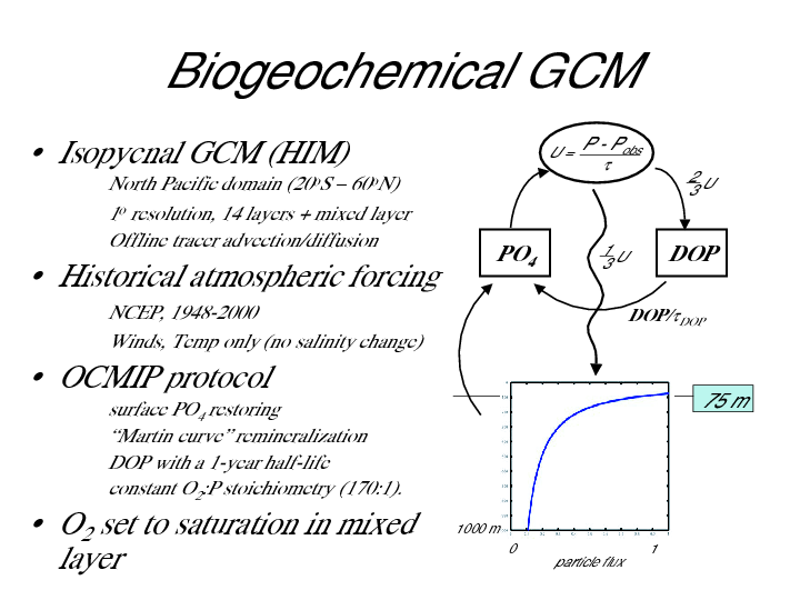
Ocean circulation is computed using a GCM that is based on the Hallberg Isopycnal Model (HIM). The model is configured for a North Pacific domain from 20°S to 60°N with 14 isopycnal layers and a horizontal resolution of 1 degree. Isopycnal layers outcrop at the surface into a Kraus-Turner mixed layer with spatially variable density. The interaction between isopycnal layers and the mixed layer is mediated by a buffer layer, through which winter mixed layer properties are detrained onto isopycnal surfaces. Circulation fields are derived from integrations forced by interannually varying atmospheric winds and surface air temperatures from NCEP reanalyses between 1948- 2000. Changes in net air-sea fresh water flux (E-P) are not included in the variable forcing, and model sea surface salinity is restored to climatological values [Levitus et al].
Time-dependent tracer distributions are computed in an offline advection/diffusion routine using monthly averaged circulation fields from the GCM. The distribution of four tracers is determined: phosphate (PO4), dissolved organic phosphorus (DOP), O2, and ideal age. DOP and PO4 are used to diagnose O2 fluxes associated with the biological pump (see below), and ideal age is computed to provide a measure of the time elapsed since a water parcel was last at the surface. All tracers are diffused along isopycnal surfaces using an eddy diffusion coefficient of 2000 m2/s. Diapycnal mass fluxes include a diffusive flux based on a constant diapycnal diffusivity of 0.1 cm2/s. Within 5 degrees of the open boundaries of the model domain, PO4 and O2 are restored toward climatological values. We integrate all tracer distributions to a near-steady state (300 years) using mean circulation fields. Tracer distributions from the steady state integration are then used as initial conditions for the variable forcing simulation, which integrates tracer distributions for another 52 years (1948-2000) using the variable circulation derived from historical atmospheric forcing.
The sources and sinks of biogeochemical tracers are computed using parameterizations based on the Ocean Carbon Model Intercomparison Project (OCMIP) (see Figure 1). In the OCMIP protocol, biological organic matter production is diagnosed by restoring model PO4 toward climatological values in the upper 75 m, with a restoring time scale of 30 days. Of the total organic matter production, two thirds is converted to DOP, which is advected and diffused and decays back to PO4 with a half-life of one year. The remaining one third is exported as sinking flux, which is instantly remineralized to PO4 with depth using a standard Martin curve . The production and remineralization of organic phosphorus pools produces and consumes O2 in a constant stoichiometric O2:P ratio of -170 mol O2/mol P. Mixed layer O2 concentrations are fixed at their (time-varying) saturation values.
The surface PO4 fields used to compute organic matter export are constant throughout the simulation. However, export flux diagnosed through nutrient restoring can vary due to changes in nutrient supply. If the supply of PO4 to surface waters increases, biological production must also increase in order to maintain constant observed surface PO4 concentrations. This parameterization of the biological pump therefore represents only those biological changes that are associated with changes in nutrient supply. It is possible that changes in biological export production over the past few decades also resulted in a net change in surface nutrient distributions. Since there is little reliable data about whether or how surface nutrients changed in the late 20th century, we make the conservative assumption that they have not.
Figure 1 - Model overview and schematic.
We perform 3 simulations. In the first (see var_ocmip_h2000_new.cdf), all sources of O2 variability are present. In two additional simulations, causes of O2/AOU variability are selectively removed, allowing us to isolate and characterize the contribution of individual processes to total O2 changes.
Because local changes in AOU are the result of several processes integrated over the history of a water parcel, we begin by considering the AOU along an isopycnal surface, which can be written as the sum of a preformed AOU (AOUo) defined just below the mixed layer, and the total O2 consumption since the water left contact with the mixed layer:
AOU = AOUo + ∫ OUR*ds/v (equation 1)
where OUR is the O2 utilization rate, which is integrated along each displacement, ds,
of the water parcel as it is transported with velocity, v. The second term on the right hand
side therefore integrates the spatially and temporally varying O2 consumption along
the path of the circulation, whose direction and speed are also spatially and temporally variable.
Preformed AOU is defined at each grid point where an isopycnal layer intersects the mixed layer. This is because while the mixed layer is assumed saturated (AOU=0), the AOU on an isopycnal surface lying just below the mixed layer depends on the degree of exchange with (i.e. ventilation by) the mixed layer. If the detrainment of waters from the winter mixed layer onto an isopycnal surface is large, AOUo will be brought close to zero. If the mixed layer is relatively isolated from the underlying isopycnal surface, the preformed AOU could be much larger than zero.
From equation 1, we can see that changes in AOU can be caused by changes in its preformed value (AOUo), changes in OUR, or changes in the speed (v) or pathway (ds) of circulation. These contributions to total AOU change can be written schematically (differentiating equation 1) as:
         ΔAOU = ΔAOUo + OUR*Δcirc + ΔOUR*circ
              = ΔAOUvent + ΔAOUcirc + ΔAOUbio                           (equation 2)
The first term on the right hand side (ΔAOUo) represents a change in preformed AOU and is therefore
associated with changes in the transfer of O2-rich waters across the base of the
mixed layer. We refer to this term as a ventilation AOU change (ΔAOUvent). The second term
represents an AOU anomaly caused by a change in the circulation, which transports water masses
along altered paths (or with altered rates) through the climatological OUR field. We refer to this
term as the circulation AOU change (ΔAOUcirc) since it is due to the direct effect of changes in
water mass location and transport. The last term represents the integrated AOU anomaly due to a
change in the distribution of OUR. We refer to this as a biological AOU change (ΔAOUbio). It is
worth noting that changes in OUR can be caused by both changes in export flux and by changes in the
depth of an isopycnal surface. Thus, the heaving or shoaling of isopycnal surfaces can alter the
OUR on that isopycnal. While not biological in origin, this effect is included by construction in ΔAOUbio.
We have performed two additional simulations in which various terms in equation 2 are eliminated. By removing individual sources of AOU variability, we can characterize the spatial pattern of AOU changes attributable to each individual process. In order to remove biological AOU changes we perform a second integration (see var_ocmip_h2000_specjo2.cdf) with the same variable circulation, but this time using the climatological (monthly varying) OUR field diagnosed from the equilibrium spin-up. Holding the pattern of OUR constant through time on each isopycnal surface removes the effect of changes in biological O2 consumption, leaving only ventilation and the direct circulation effects as factors in the variation of O2/AOU.
In a third simulation (see var_ocmip_h2000_vent_test.cdf), we remove the influence of both ventilation and biological changes on O2/AOU values by holding both OUR and AOUo constant at their climatological values. Changes in AOUo are removed by forcing the AOU on each isopycnal surface to remain at its monthly climatological value wherever that surface intersects the mixed layer either in the climatological mean state or at any time during the variable circulation run. For example, the region over which a given isopycnal surface lies at the base of the mixed layer could shift poleward as a result of warming. This would produce a new region of isopycnal/mixed layer interaction to the north of the climatological outcrop. The effect of increased ventilation on O2/AOU in that region is eliminated in this simulation, by forcing AOU at the local isopycnal/mixed layer interface to remain at climatological values. Similarly, equatorward of the climatological outcrop the isopycnal layer will lose contact with the mixed layer, as less dense water intercedes between them. The impact on O2 of the resulting decrease in ventilation is again prevented, by maintaining the AOU at its climatological value at that location. This manipulation removes the effect of changes in the location and/or strength of ventilation, assuring that changes in the detrainment of mixed layer water onto an isopycnal surface will have no effect on the preformed AOU. Holding constant both OUR and AOUo therefore yields AOU changes that result solely from the direct influence of circulation changes.
Table 1 summarizes the 3 simulations and the sources of AOU variability in each one. The contribution of biology, ventilation, and circulation to the total AOU change can thus be separated as follows:
          ΔAOUcirc =  ΔAOU(Experiment 3)
          ΔAOUvent =  ΔAOU(Experiment 2) -  ΔAOU(Experiment 3)
          ΔAOUbio  =  ΔAOU(Experiment 1) -  ΔAOU(Experiment 2)
where the experiment names are related to output files as follows:
          Experiment 3 = var_ocmip_h2000_vent_test.cdf
          Experiment 2 = var_ocmip_h2000_specjo2.cdf
          Experiment 1 = var_ocmip_h2000_new.cdf
By construction, the sum of AOU anomalies (relative to an arbitrary reference time) from these
three processes yields the total AOU change.
Each variable name is preceded by mn_ which indicates that all variables are annual mean values. The fields are defined on a 1 degree grid from 20°S to 60°N, from 90°E to 70°W (80 x 200 grid points). The vertical coordinate is potential density, with the top two layers representing the mixed and buffer layers (see above). Densities of the 14 isopycnal layers are 21.25, 21.75, 22.5, 22.8, 23.25, 24.25, 24.75, 25.75, 26.2, 26.6, 27, 27.35, 27.6, 27.8 sigma-theta.
| Variable Name | Variable description/definition |
| mn_h | Thickness of each isopycnal layer (meter) |
| mn_oxygen | Dissolved oxygen (µmol/l) |
| mn_o2sat | Oxygen saturation concentration (µmol/l) |
| mn_phos | Phosphate concentration (µmol/l) |
| mn_pflux | Phosphate export, integrated over the top 75 m (mmol/m2/sec) |
| mn_age | Ideal age tracer (years) |
| mn_jo2 | Biological oxygen utilization rate (OUR) (mol/m3/sec) |
| mn_dop | Dissolved Organic Phosphorus (DOP) concentration (µmol/l) |
| mn_pobs | Observed phosporus (µM) |
| mn_o18 | delta-18O of O2 (permil) |
C. Deutsch, L. Thompson, and S. Emerson. 2005. Attributing the causes of North Pacific Oxygen Change. in prep.