5 Upper Ocean Modeling at NCAR

Scott Doney

Climate and Global Dynamics

National Center for Atmospheric Research

Boulder, CO 80307

The bulk of the primary and new production in the worlds ocean is generated either in the ocean planetary boundary layer (PBL) or underlying seasonal thermocline. The most relevant physical phenomena for understanding the patterns and timing of biological productivity, therefore, are often the seasonal variability in the PBL depth, which also affects the mean irradiance observed by phytoplankton, and the turbulent fluxes of nutrients across the PBL bottom boundary and through the seasonal thermocline. A one-dimensional, coupled biological--physical model has been designed at NCAR as the first part of a longer term project for developing a global ocean biological modeling capability. The coupled modeling effort has been guided by two criteria: the model should capture the essential characteristics of the marine ecosystem under consideration while remaining simple enough, both conceptually and computationally, to allow for incorporation into basin and global-scale ocean circulation models. Here I present model results from a simulation from the oligotrophic Sargasso Sea, with emphasis on understanding the response of the phytoplankton and nutrient profiles to physical forcing (e.g. wind mixing, convection) over seasonal time periods.

Our basic, underlying philosophy for the coupled modeling work is that the essential physical processes of the ocean PBL must be captured correctly as a prerequisite if one wishes to accurately model the behavior of an upper ocean ecosystem. The physical component of the coupled model is a non-local, turbulent mixing scheme developed by Large et al. (1994) to simulate the oceanic planetary boundary layer (PBL) and seasonal thermocline. The conceptual basis for the model, referred to as the K-profile parameterization (KPP), arises from two basic premises: 1) mixing processes in the PBL are inherently non-local (i.e. the mixing at any point in the boundary layer is driven by the generation of turbulence at the surface and bottom of the PBL) and 2) eddy diffusivity profiles in a PBL, either atmospheric or oceanic, are similar in shape when the appropriate scalings, involving the boundary layer thickness and the turbulent forcing terms (e.g. surface wind stress and buoyancy flux), are applied. The development of the KPP model has been based to a large degree on the more extensive modeling and observational work available in the atmospheric PBL community.

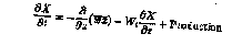
The time evolution for a mean property X (momentum or scalar) at any depth z in the model is given by:

(1)

where is the mean turbulent flux of X given by the model and Wt is the total vertical velocity, the sum of the advective and particle sinking velocities. Solar adsorption and biological

processes are included in the production term; for the velocity components U and V, this term accounts for the Coriolis effect. The model itself consists of three components that, in turn, calculate the vertical profile of , the depth of the PBL h, and the diffusive fluxes below the PBL in the seasonal and main thermoclines.

The turbulent fluxes in the PBL are formulated in terms of an eddy diffusivity

Kx(z) and a counter-gradient term:

0 < z < h

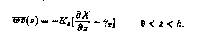(2)

The counter-gradient term stems from atmospheric observations and model results that show significant turbulent heat fluxes in convective PBLs over regions of zero mean temperature gradient, reflecting the asymmetric and non-local nature of turbulence in a convective PBL. The shape of K(z) with depth is fixed and the magnitude increases with surface wind stress and boundary layer depth. This result follows from the argument that mixing is dominated by the largest-scale eddies in the boundary layer, and a deeper PBL can maintain larger and stronger turbulent eddies. The eddy diffusivity is also enhanced in unstable conditions when the surface buoyancy flux is out of the ocean. The depth of h varies with both surface forcing and the mean oceanic buoyancy and velocity profiles, and is determined prognostically based on a bulk Richardson number stability criteria (Large et al., 1994). Three distinct mixing processes are considered in the interior below the PBL: shear instability, internal wave breaking, and double diffusion. In general the resulting interior diffusivities are small, on the order of 0.1-0.2 cm2 s-1.

The behavior of the KPP physical model has been validated against oceanic observations over a range of timescales (diurnal to inter-annual) and environments (subtropical to subpolar North Pacific) (Large et al., 1994; Large and Crawford, 1994). In general, the KPP model appears to perform at a comparable or slightly better level relative to the other available one-dimensional models. In particular, the model demonstrates a significant improvement in the exchange of properties between the mixed layer and thermocline. The model temperature and velocity fields are shown in Figure 5.1 for simulation of an episodic wind or storm event. Note that following the wind event there has been a significant downward transport of heat and momentum into the seasonal thermocline, despite the relatively small change in the apparent mixed layer depth.

Following a long modeling tradition in the biogeochemical community (e.g. Fasham et al., 1990), biological constituents in the coupled model are treated as equivalent scalar concentrations of nitrogen. Photosynthesis by autotrophic organisms forms the foundation of the euphotic zone ecosystem, and a key element in any coupled, upper ocean model, therefore, is the phytoplankton biomass and the associated mechanisms that control the biomass and primary production rate (e.g. irradiance and nutrient limitation, grazing). Because the rate of new production is determined over much of the ocean by the supply NO3- from below the euphotic zone, a model of long-term behavior must, at a minimum, also include vertical transport of inorganic nitrogen by upwelling and physical mixing, sinking of detrital particulate organic nitrogen, and regeneration of nitrogen in the aphotic zone. At present these processes are

Figure 5.1: KPP simulations of temperature and velocity to an episodic wind event. The applied surface wind stress starts from zero, peaking at hour 10, and rotates at the inertial frequency. Note the significant downward transport of heat and momentum into the seasonal thermocline following the wind event.

Figure 5.2: Schematic of the four component (PZND) biological model used in the coupled model work.

incorporated into the coupled model using a simple, four component system---phytoplankton (P), zooplankton (Z), nutrients (N), and detritus (D) (PZND model)---outlined schematically for a single grid level in Figure 5.2. Additionally, the model allows for variation in the chlorophyll to N ratio of the phytoplankton pool in response to their nutrient and light status.

The physical simulation for the Sargasso Sea was generated with smooth, harmonic forcing for wind stress and heat flux based on climatology. The simulations (Figure 5.3) show the characteristic deep convective mixing during winter and the shallow mixed layer and seasonal thermocline during the summer. The seasonal SST cycle is also of the correct amplitude based on climatology. In most locations, the heat balance over the annual cycle is not closed locally, and in order to satisfy the annual heat balance an advective flux is prescribed. The manner in which this heat is added to the model can greatly modify the resulting physical solution. Previous 1-D physical models for the Bermuda region have required a relatively high vertical diffusivity for temperature ~1cm2 s-1 to match the observed seasonal cycle (Musgrave et al., 1988). Trade-offs exist, however, among vertical diffusivity, down-welling velocity and horizontal advection, and the annual thermal cycle can be simulated equally well with a low diffusivity, which influences the nutrient flux into the euphotic zone during summer.

The coupled biological simulations of chlorophyll (Figure 5.4) show a spring bloom shortly after the mid-winter injection of nutrients into the mixed layer by entrainment. The spring bloom rapidly depletes surface nutrients and results in a large, downward flux of nitrogen from turbulent mixing of phytoplankton as well as sinking detritus. A sub-surface chlorophyll maximum develops during the spring and summer at the top of the nitricline; the sub-surface maximum is primarily a result of increased chlorophyll to N ratios at that depth rather than a build-up phytoplankton biomass. Note that the spring bloom and the summer, sub-surface maximum appear to be separate structures. The model predicted primary production values are similar to those found in the JGOFS BATS data for spring and summer, and fall off during late summer, perhaps due to a de-coupling of the nitrogen and carbon cycles.

Work is currently underway to incorporate both the KPP physical model and coupled biological model into a global, three-dimensional circulation model of the GFDL class.

Figure 5.3: Annual cycle in temperature (°C) versus depth and time for the Sargasso Sea using smooth, climatological surface forcing.

Figure 5.4: Simulated chlorophyll (mg Chl m3) versus time and depth from the coupled model for the Sargasso Sea.