J-LAS and Merged Data Product Tutorial

Cyndy Chandler, US JGOFS DMO

from October 2001 presentation

at Woods Hole Oceanographic Institution

J-LAS is the US JGOFS customized version of the Live Access Server (LAS) developed at NOAA/PMEL by Steve Hankin, Jon Callahan and Joe Sirott. As of October 2001, this software is still a Beta release.

To begin: start up an Internet browser (Netscape or Internet Explorer) and

open the J-LAS class start page:

URL is http://usjgofs.whoi.edu/datasys/JLAS_class/J-LASclass.html

Select one of the links from the J-LAS class page.

Some J-LAS Hints

There are three distinct areas in the main J-LAS screen. The title bar across the top includes a server title in the center (US JGOFS Process Studies) and four link buttons to the right.

Help: generic LAS help	Options: modify Ferret settings
Home: will go to US JGOFS	Ferret: goes to Ferret Home

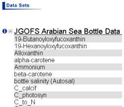Data sets are listed in the left frame. Click on the name of a data set to expand it and view a list of available variables. Click on a variable name to select that variable within the expanded data set. The variable name should appear in the frame to the right. [Single variable only in this release.]

Select to display documentation window.

ie. C_toN = Carbon to Nitrogen ratio; US JGOFS Arabian Sea Process Study Niskin samples

You can modify the data selection by adjusting spatial and temporal bounds:
Latitude, Longitude, Depth and Time ranges (XYZT respectively).

You may change the viewing plane.

Select from: XY: Longitude v. Latitude
XZ: Longitude v. Depth (view from East)
YZ: Latitude v. Depth (view from South)

You may also wish to select a different product from the drop down list at the bottom of the screen. Current choices include a variety of GIF images and download formats:

XY pie plot (GIF) to get an indication of sample locations on lat/lon map

XZ pie plot (GIF) for longitudinal depth section

YZ pie plot (GIF) for latitudinal depth section

XZ [YZ] Gaussian filled plot (GIF); algorithm used is a Gaussian weighted mean of input points where weights vary with Gaussian decay and independent cutoff value.

It is also possible to download the data in plain text format or as a NetCDF file.

When you have made desired adjustments to various ranges, choose Get Data to view your data (usually as a GIF image in a new window).

The next few pages are printed from the generic LAS Help screen. Try some things out, have fun, ask questions when you get stuck. I am very interested in knowing what you like about the interface and any suggestions you might care to share. Please keep in mind you are using a Beta release version. (cchandler@whoi.edu)